Lecture 2: k-Nearest Neighbors

From similarity to learned compatibility

Problem formulation, neighborhood classification, geometry, teammate matching, distance learning, and evaluation.

Nearest-neighbor methods begin with a practical problem and a simple assumption: proximity under the chosen representation and distance should support useful predictions. Understanding the model means tracing that assumption through data collection, feature construction, eligibility, geometry, and evaluation.

Learning goals

By the end of this lecture, you should be able to:

start from a practical decision and formulate its examples, features, target, eligibility rules, and evidence of success;
apply k-NN classification using a neighborhood, a voting rule, and a justified choice of $k$;
explain how the representation and distance encode the model’s proximity assumption; and
translate a human preference into a logical constraint and a loss for distance learning.

Begin with the problem

Machine learning starts with a decision we want to improve. The algorithm comes later.

Design note

A precise problem statement prevents a common failure: optimizing a clean mathematical target that does not correspond to the real decision.

A brief labeled example

Begin with the problem: predict whether a listener will like a new track using historical likes and dislikes. Represent each track as a feature vector such as

\[ \mathbf{x} = \begin{bmatrix} \text{tempo} & \text{energy} & \text{danceability} & \text{acousticness} & \cdots \end{bmatrix}^{\!\top} \in \mathbb{R}^d, \]

with an observed label $y\in\{0,1\}$, where $1$ denotes “liked.” The data are

\[ \mathcal D=\{(\mathbf{x}_i,y_i)\}_{i=1}^{n}. \]

For an unseen track $\mathbf{x}_\star$, the output is a prediction $\widehat y(\mathbf{x}_\star)$. The hat matters: $y$ is observed evidence; $\widehat y$ is what the model predicts.

Using k-NN adds a modeling assumption: proximity should support good predictions. Data collection and feature design are part of that assumption because they determine which forms of proximity the model can see.

The k-nearest-neighbor rule

Let $\mathcal D=\{(\mathbf{x}_i,y_i)\}_{i=1}^{n}$ and let $d(\cdot,\cdot)$ be a dissimilarity rule. For a query $\mathbf{x}$, sort the training indices so that

\[ d(\mathbf{x},\mathbf{x}_{(1)}) \le d(\mathbf{x},\mathbf{x}_{(2)}) \le \cdots \le d(\mathbf{x},\mathbf{x}_{(n)}). \]

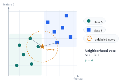
The neighborhood index set is

\[ \mathcal N_k(\mathbf{x})=\{(1),(2),\ldots,(k)\}. \]

This order-statistic definition makes the computation transparent. If points tie at the $k$th distance, a deterministic rule is still required.

A binary scatterplot with a query point and its three nearest neighbors highlighted. — Figure 1: A synthetic binary example. The query’s three nearest points contain two teal circles and one blue square, so unweighted $k=3$ predicts the teal class. The geometry, not the plotting axes alone, determines the neighborhood.

Classification and distance weighting

For class labels $c\in\mathcal C$, unweighted k-NN classification predicts

\[ \widehat y(\mathbf{x}) = \operatorname*{arg\,max}_{c\in\mathcal C} \sum_{i\in\mathcal N_k(\mathbf{x})} \mathbb{1}[y_i=c]. \]

Closer neighbors can receive more influence. With nonnegative weights $a_i(\mathbf{x})$, a common choice is

\[ a_i(\mathbf{x}) = \frac{1}{d(\mathbf{x},\mathbf{x}_i)+\varepsilon}, \qquad \varepsilon>0. \]

The weighted classifier replaces vote counts with weighted counts. The small $\varepsilon$ prevents division by zero, although exact matches deserve an explicit policy.

What does $k$ control?

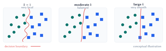
In classification, $k$ controls how local the vote is. A small $k$ follows individual observations closely; a larger $k$ aggregates evidence across a wider neighborhood.

Three classification sketches compare increasingly smooth decision boundaries as k grows. — Figure 2: Conceptual effect of $k$ in classification. Small neighborhoods react strongly to individual observations; larger neighborhoods average across a wider region. Select $k$ with validation data, not by visual preference.

Table 1: The appropriate $k$ is data-dependent. Cross-validation estimates which neighborhood size generalizes.

Choice	Boundary behavior	Main advantage	Main risk
$k=1$	Highly local and irregular	Preserves fine structure	Sensitive to noise and mislabeled points
Moderate $k$	Smooths nearby evidence	Often balances bias and variance	Must be tuned to density and sample size
Large $k$	Approaches a global vote	Stable under local noise	Erases local structure and favors common classes

Odd $k$ is not a complete tie policy

An odd $k$ reduces vote ties only for binary classification when the neighborhood itself is unambiguous. Multiclass votes, equal distances at the cutoff, and duplicate points can still tie. Use a documented rule such as distance-weighted voting, a fixed class order, or inclusion of all points tied at the boundary.

The geometry is the model

The k-NN rule assumes that nearby examples are useful for prediction, but the distance decides which examples count as nearby. Changing the dissimilarity can change every neighbor. In a zero-shot system, this is a substantive modeling assumption.

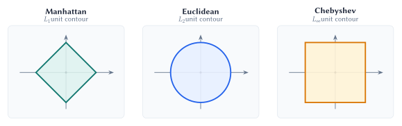
Let $\Delta_j=x_j-z_j$. The Minkowski family is

\[ d_p(\mathbf{x},\mathbf{z}) = \left(\sum_{j=1}^{d}|\Delta_j|^p\right)^{1/p}, \qquad p\ge 1. \]

Euclidean distance uses $p=2$, Manhattan uses $p=1$, and the limit $p\to\infty$ gives Chebyshev distance.

Unit contours compare Manhattan, Euclidean, and Chebyshev distance in two dimensions. — Figure 3: Unit-distance contours in two dimensions. A point on each contour is exactly one unit from the center under that metric. Different contours imply different neighbor orderings.

Four common rules

Table 2: Metric choice should follow the semantics of the features and the downstream decision.

Rule	Definition	Useful when	Caution
Euclidean	$\sqrt{\sum_j\Delta_j^2}$	Straight-line proximity is meaningful; large coordinate gaps should count strongly	Sensitive to outliers and irrelevant coordinates
Manhattan	$\sum_j\|\Delta_j\|$	Coordinate-wise deviations add; sparse or robust comparisons are desirable	Axes remain equally weighted by default
Chebyshev	$\max_j\|\Delta_j\|$	The largest mismatch acts like a deal-breaker	Ignores improvement on nonmaximum coordinates until the maximum changes
Cosine dissimilarity	$1-\dfrac{\mathbf{x}^{\top}\mathbf{z}}{\lVert\mathbf{x}\rVert_2\lVert\mathbf{z}\rVert_2}$	Direction or relative pattern matters more than magnitude	Undefined for a zero vector; $1-\cos$ is not generally a mathematical metric

Why cosine helps with document counts

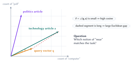
Suppose articles are represented only by counts of the words “computer” and “poll.” A long technology article and a short technology query may point in nearly the same direction even when their Euclidean distance is large. Cosine similarity measures that direction:

\[ \operatorname{cosim}(\mathbf{x},\mathbf{z}) = \frac{\mathbf{x}^{\top}\mathbf{z}} {\lVert\mathbf{x}\rVert_2\lVert\mathbf{z}\rVert_2} =\cos\theta. \]

Here $\theta$ is the angle directly between the two nonzero vectors at their shared origin.

Figure 4: The marked angle $\theta$ lies between the query vector and the technology-article vector. Their directions are similar even though their lengths and Euclidean separation differ.

Validity requires a domain argument

A metric can be mathematically well-defined and still encode the wrong domain assumption. A useful task-specific score may also violate symmetry or the triangle inequality. Name the object honestly: distance, dissimilarity, or compatibility cost.

Case study: zero-shot teammate matching

The lecture dataset contains 41 survey responses. An NLP extraction step maps each response to eight numerical axes on a nominal $[-1,1]$ range. Treat yourself as the fixed query. The missing outcome for each candidate is

\[ y_i=\mathbb{1}\{\text{student $i$ works well with me}\}. \]

Those collaboration outcomes do not yet exist. The first system is nearest-neighbor candidate ranking under designed assumptions.

Role of k-NN

k-NN returns the nearest eligible candidates under the representation and scoring rule we choose. The system designer still has to define compatibility.

Representation and system roles

Table 3: The eight extracted axes. The final column is a design hypothesis, not a discovered fact.

Feature	Negative endpoint	Positive endpoint	Possible role
`theory_implementation`	Theory / mathematics	Implementation / engineering	Role coverage
`research_industry`	Research / academic	Industry / product	Context dependent
`structured_exploratory`	Structured problems	Exploratory / open-ended	Work-style alignment
`solo_collaborative`	Solo work	Team collaboration	Work-style alignment
`depth_breadth`	Deep focus	Broad interests	Context dependent
`plan_iterate`	Plan first	Iterate quickly	Work-style alignment
`data_model`	Data / analysis first	Model / algorithm first	Role coverage
`foundational_applied`	Build foundations	Applied solutions	Context dependent

The categorical team_status field serves a different purpose: it is an eligibility rule. Students choosing to work solo should be filtered out before distances are ranked. Treating eligibility as another coordinate can return operationally invalid neighbors.

Separate the layers

Representation features, eligibility constraints, and the scoring function answer different questions. Keep them explicit.

Standard metrics disagree

For the worked comparison, one anonymized profile stands in for you. The notebook ranks all eligible candidates using all eight features and keeps the top three under each rule.

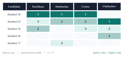
A matrix compares the top three teammate candidates under Euclidean, Manhattan, cosine, and Chebyshev scoring. — Figure 5: For the same anonymized query profile, different metrics produce different top-three lists. Student 03 is the only candidate appearing under all four rules. A dash means the candidate falls outside that metric’s top three.

The disagreement is not an implementation bug. Euclidean aggregates squared gaps, Manhattan aggregates absolute gaps, cosine compares orientation, and Chebyshev focuses on the largest coordinate gap. Each rule compresses the same profile difference differently.

What unlabeled data cannot tell us

Without compatibility outcomes, Figure 5 cannot identify a correct metric. The metric must be defended as a transparent domain assumption and later validated against feedback or collaboration outcomes.

Similarity is only one design objective

A team matcher may seek:

alignment on working approach, to reduce coordination friction;
coverage across technical perspectives, to avoid redundant strengths; and
eligibility constraints, to respect availability and stated preferences.

These objectives are not equivalent to Euclidean closeness. We can alter the geometry by learning which similarities matter from feedback or by targeting nonzero gaps for complementary roles.

Learning and designing a better ruler

Distance learning begins with a concrete failure: we prefer $A$ to $B$, but the current metric ranks $B$ closer. We turn that desired ordering into a logical condition and then a loss the machine can optimize.

A two-feature counterexample

Consider a toy $[0,10]$ profile with

\[ \mathbf{x}_{\mathrm{me}}=[5,5], \qquad \mathbf{x}_A=[5,9], \qquad \mathbf{x}_B=[7,6]. \]

The first feature is theory versus implementation; the second is coding versus mathematics. Suppose prior experience says $A$ is preferred to $B$.

Table 4: Ordinary Euclidean distance ranks $B$ closer even though the observed preference favors $A$.

Candidate	Squared gap on $x_1$	Squared gap on $x_2$	Unweighted squared distance
$A=[5,9]$	$(5-5)^2=0$	$(5-9)^2=16$	$16$
$B=[7,6]$	$(5-7)^2=4$	$(5-6)^2=1$	$5$

The human preference becomes the logical condition

\[ d_{\mathbf{w}}(\mathbf{x}_{\mathrm{me}},\mathbf{x}_A)^2 < d_{\mathbf{w}}(\mathbf{x}_{\mathrm{me}},\mathbf{x}_B)^2. \]

Give the model parameters that can satisfy this ordering with a diagonal weighted squared distance:

\[ d_{\mathbf{w}}(\mathbf{x},\mathbf{z})^2 = \sum_{j=1}^{d}w_j(x_j-z_j)^2, \qquad w_j\ge 0. \]

If every weight is strictly positive, $d_{\mathbf{w}}$ is a metric. Allowing a zero weight collapses that coordinate and yields a pseudometric.

With $w_1=4$ and $w_2=1$, the squared distances become $16$ for $A$ and $17$ for $B$. The ranking flips because agreement on the first feature is declared four times as important.

What diagonal weights can express

Positive diagonal weights learn which similarities matter. They cannot reward a nonzero feature gap, model interactions between features, or satisfy a preference when the positive example is no closer on any available coordinate.

From a preference to a learnable loss

A triplet $(a,p,n)$ records that anchor $a$ prefers positive example $p$ over negative example $n$. With margin $m>0$, the desired condition is

\[ d_{\mathbf{w}}(a,p)^2+m \le d_{\mathbf{w}}(a,n)^2. \]

Define the constraint gap

\[ g_{a,p,n}(\mathbf{w}) = d_{\mathbf{w}}(a,n)^2-d_{\mathbf{w}}(a,p)^2. \]

The condition is $g_{a,p,n}(\mathbf{w})\ge m$. The hinge loss measures how far the current weights are from satisfying it:

\[ \mathcal L(\mathbf{w}) = \max\bigl(0,m-g_{a,p,n}(\mathbf{w})\bigr). \]

Why the maximum matters. Without the outer maximum, minimizing $m-g$ would keep rewarding an already-correct triplet for making the gap arbitrarily large. Clipping at zero once the margin is met prevents this reward hacking and focuses learning on preferences that are still violated.

For an active hinge, the feature-wise gradient is

\[ \frac{\partial\mathcal L}{\partial w_j} = (a_j-p_j)^2-(a_j-n_j)^2. \]

A projected update keeps weights feasible:

\[ \mathbf{w} \leftarrow \Pi_{\mathbb{R}_{\ge 0}^{d}} \left(\mathbf{w}-\eta\nabla_{\mathbf{w}}\mathcal L\right). \]

These updates require observed preference triplets. Learned weights should be assessed on held-out feedback; satisfying the training triplets alone does not establish useful compatibility.

Complementarity requires a different objective

A maximum-gap rule can reward extreme differences even when extremes make collaboration harder. A more explicit design targets a moderate gap for role coverage.

For absolute feature gaps $\Delta_j=|x_j-z_j|$, split features into alignment set $S$ and coverage set $C$:

\[ \begin{aligned} L_{\mathrm{align}} &=\operatorname{mean}_{j\in S}\Delta_j^2,\\ L_{\mathrm{cover}} &=\operatorname{mean}_{j\in C}(\Delta_j-\tau)^2,\\ C(\mathbf{x},\mathbf{z}) &=\alpha L_{\mathrm{align}} +(1-\alpha)L_{\mathrm{cover}}. \end{aligned} \]

In the worked example, the alignment set contains structured/exploratory; the coverage set contains theory/implementation and data/model. We use $\tau=0.6$ and $\alpha=0.5$.

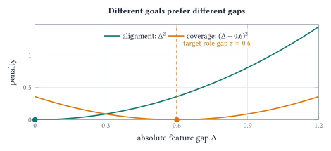
Two penalty curves show alignment minimized at zero gap and role coverage minimized at a target gap of 0.6. — Figure 6: Alignment has its minimum at zero gap; role coverage has its minimum at the chosen target $\tau=0.6$. The parameters expose assumptions that can be debated and tested.

Compatibility cost

On a coverage feature, zero gap can receive a penalty, so identity of indiscernibles fails. The score ranks potential partners for one query; it does not prove compatibility or optimize an entire team’s composition.

Evaluation belongs to the whole pipeline

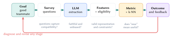
An apparently simple neighbor lookup rests on a chain of assumptions: the problem is framed correctly, data collection captures relevant evidence, the representation preserves it, eligibility is valid, and the chosen distance makes proximity useful. When outcomes are poor, diagnose the whole chain. The choice of $k$ is only one possible source.

A pipeline connects problem framing, survey questions, feature extraction, eligibility, distance, ranking, and outcome evaluation. — Figure 7: The teammate-matching pipeline. Evaluation feeds back to every stage: the goal, questions, extraction, eligibility, and geometry can all be failure sources.

Match evaluation to the task

Table 5: Choose a split and measurement that reproduce the future decision.

Setting	Validation unit	Useful measurements	Leakage to avoid
Supervised classification	Future examples or entities, depending on deployment	Accuracy, balanced accuracy, precision/recall, calibration	The same entity or a near duplicate in train and test
Candidate ranking	Query with judged relevant items	Recall@$k$, precision@$k$, mean reciprocal rank, NDCG	Using relevance feedback from evaluation queries to design the metric
Team matching	Pair or team outcome after collaboration	Preference satisfaction, acceptance rate, project outcome, subgroup diagnostics	Using evaluation preferences to design or fit the score

For supervised k-NN, tune preprocessing, the distance rule, weighting, and $k$ inside cross-validation. For teammate ranking, compare transparent baselines and gather outcome feedback before presenting rankings as learned recommendations.

Baseline ladder

Start with a simple eligible-candidate baseline, then compare unweighted Euclidean, alternative metrics, weighted k-NN, and only then a custom learned or complementary score. Each extra degree of freedom should earn its complexity on held-out evidence.

Diagnose failures at the right layer

Table 6: A failure map for the full pipeline. Model tuning is only one possible response.

Layer	Assumption	Diagnostic	Possible intervention
Goal	“Good teammate” has an operational meaning	Compare stakeholder definitions and downstream outcomes	Reframe the target; separate compatibility, coverage, and logistics
Survey	Questions capture relevant, answerable traits	Reliability checks; missingness; interviews; outcome correlations	Revise questions or collect direct behavioral evidence
Extraction	Text becomes faithful numerical features	Human rubric audit; repeated extraction; subgroup error analysis	Calibrate prompts or rubrics, add examples, or replace the extractor
Eligibility	Returned candidates are actionable	Count invalid recommendations and constraint violations	Filter first; encode hard constraints outside the distance
Geometry	Lower score corresponds to better pairs	Neighbor inspection; counterexamples; held-out preferences	Reweight, learn a metric, or redesign the score
Outcome	The ranking improves collaboration	Prospective evaluation and qualitative follow-up	Revisit upstream layers; retuning $k$ alone may not help

Lecture summary. Practical k-NN starts from the problem: trace the assumption that proximity predicts well through data collection, representation, eligibility, distance, and evaluation, then convert observed ranking failures into constraints and losses the model can learn from.

Candidate	Squared gap on \(x_1\)	Squared gap on \(x_2\)	Unweighted squared distance
\(A=[5,9]\)	\((5-5)^2=0\)	\((5-9)^2=16\)	\(16\)
\(B=[7,6]\)	\((5-7)^2=4\)	\((5-6)^2=1\)	\(5\)